Analysis for Genetic Programming Maze Marchers
The Speed Problem: I must preface my analysis with an apology regarding the meager quantity of data that I was able to obtain. To be certain that the conclusions being drawn about the behavior of the model are correct, one desires to have a large quantity of data. Obtaining the data is unfortunately a slow process. A single simulation run on the model can take 10 minutes, or more, to find a solution. Some runs will never find a solution, and will have to be cut off after some number of generations (I will note what the cutoff generation is in each of the experiments below). This means that my BehaviorSpace experiments could take 3 or 4 hours to complete. Because of this slowness of collecting data, and because of the number of parameters in the model, I didn't have time to examine more than one dimension of the parameter space at a time. Instead, I started with a set of default values for the parameters:
population-size = 50
initial-code-max-depth = 10
branch-chance = 0.9
clone-chance = 20
crossover-chance = 70
mutate-chance = 10
maze-file = “maze0.txt"
(fix-random-seed? = false for all
experiments, for obvious reasons)
These choices for default values were somewhat arbitrary -- I chose them because I believed them to give fairly decent results. Then, I varied each of these variables individually, while holding the others fixed. Even so, I was often limited by time constraints to do only a few repetitions at each variable setting. Since genetic programming is a stochastic mechanism, this leaves some uncertainty about whether trends in the data are attributable simply to random noise, or whether they have a real basis. Also, if time were not so limited, I would have liked to do some multidimensional analysis of the genetic operation probabilities (crossover vs. mutation vs. cloning), to see if I could learn anything about how they relate to each other.
Format of the results:
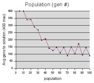
For each experiment, I created two graphs. The first shows the average number of generations before the solution is found. For this graph, it is important to understand that since there is a maximum cutoff M, if no solution is found in M generations, the run will report M as the solution generation number (even though we don't know whether or not a solution will be found in generation M+1, M+1000, or never). If this is confusing, it will be clearer when you look at some of the graphs.
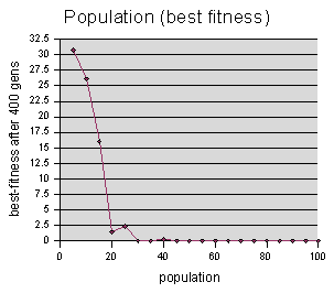
The second graph shows the best-fitness achieved. If the solution is found, then the best-fitness is 0. If no solution is found in the M generations, then the best-fitness value of generation M is returned.
These two graphs are somewhat complimentary in nature. For instance, if every run finds a solution, then the best-fitness graph will be flat zeros, but the “generations to solution” graph will show us how long it took each run to find the solution, and so we can judge the parameters on that basis. On the other hand, if no run finds a solution, then the “generations to solution” will be flat Ms, but we can use the “best-fitness” graph as an estimate of how close the runs might have been to finding a solution.
 |
 |
The
population data were sampled at
intervals of 5 units, with each run repeated 5 times. Maximum cutoff
M = 400 generations.
Note the jagged lines lines in the “gen #” graph after 55. This behavior of the graph just screams out “random noise,” because there is no reason that a population of 70 should do considerably better than both 65 and 75, except for random chance. If enough samples could be taken, and averaged, we would expect this graph to smoothen out.
We can also observe here the effects I mentioned earlier of runs reporting M (400) when they hit the cutoff. On our “gen #” graph, the value for population=5 should be much higher than population=10, but instead they are both at 400. The “gen #” should continue to climb higher as we move left, reaching toward infinity when population= 0 (since no solution can be found when there are no codeturtles to find it).
The overall trend here is that a larger population gives better results for genetic programming. Intuitively, this makes sense -- the more codeturtles you have, the more likely it is that one of them is going to find a solution, even if their actions were entirely random. At least for this model, it appears that once you reach a population of about 50, the benefit of adding more codeturtles decreases. This is interesting, because for many genetic programming problems, researchers use populations of 5000 or more (I was unable to test with such large numbers, on account of the inefficiency of the model.)
There is an important factor that my charts do not take into account -- namely, time. What we are really interested in minimizing is the time that it takes to find a solution, not the number of generations. Unfortunately I did not measure the actual time that it took for these runs to complete. (Even if timing had occurred to me, there could have been some difficulties with it, because not all of the experiments were run on the same computer, and also sometimes the experiments were running in the background, and so might be getting less CPU time, etc.) The reason I bring it up-- suppose that it averages about as many generations with 50 turtles as it does with 100 turtles. Which should we choose? Well, running 100 turtles takes about twice as long in each generation, so 50 would be much better. I created another graph that scales the “average generations to solution” by the population size, which would gives us an estimate of the relative time taken to find the solution.
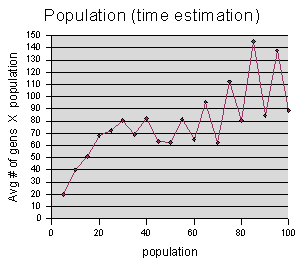
This chart leads us to believe that
perhaps the quickest way to get to the solution is to use a
population size between 40 and 60. This is just a guess, again,
since the roughness of our graph shows that the randomness factor is
significant.
(At first glance, it may appear that the quickest way is to use population size 5, but it turns out that we need to throw out all of the data points to the left of about 20, because their “average generations to solution” is underestimated on account of using the 400 generation cutoff value. We can see from the “best fitness” graph above, that populations of 15 or less rarely even got close to the solution.)
 |
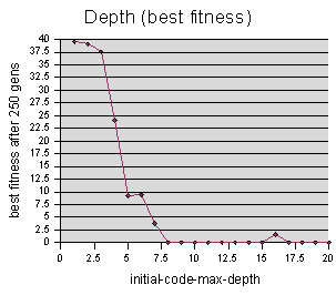 |
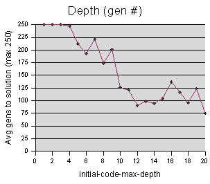
The initial-code-max-depth data was sampled at intervals of 1 unit, averaging 3 repetitions per sample value. The maximum cutoff M = 250 generations.
Somewhat similar to our population graph, we find that in order to get good results, we should start with a certain code depth, but increasing it beyond 14 or so appears unnecessary. There are actually two explanations for this. The first is that starting codeturtles off with longer code, beyond a certain length, doesn't really benefit the simulation. The second, and less obvious, is that it could be that increasing the code depth limit beyond a certain level doesn't actually change the length of the code. The length of the code is also limited by the branch-chance, and it could be that getting depths beyond 14 is improbable, based on the diminishing branching factor.
 |
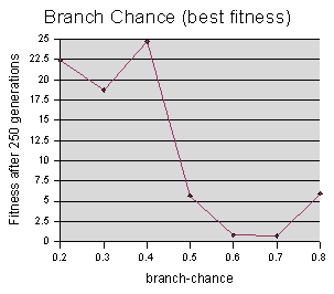 |
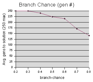
Both graphs suggest that higher branch chances (which means longer starting code) yield better performance. Although the best-fitness value begins to go back up at branch-chance = 0.8, I believe this is a fluke, caused by a bad luck run, since the # of generations graph continues to drop. (This experiment accidentally only sampled up to 0.8, when it should have also sampled 0.9, and I haven't had time to run it again.)
 |
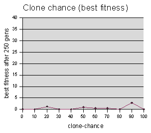 |
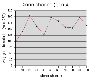
Clone-chance data were sampled at intervals of 10, averaging 5 runs per sample value.
Since almost all runs ended in a
solution, the “best fitness” graph for this one is
uninteresting. Furthermore, the “gen #” graph appears
very noisy. No trends are clear -- one might hazard a guess that the
genetic operation of cloning is superfluous to genetic programming,
and possibly even harmful. But without more data, conjecturing seems
somewhat frivolous. Also, even if it doesn't have a large effect
with this particular parameter set, it could be that it is crucial
when you have a different size population, a different chance of
crossover, a different maze, or even an entirely different problem. in
fact, drawing conclusions about genetic programming as a whole,
simply on the basis of this maze model, is surely a foolish idea.
 |
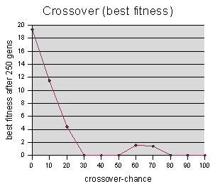 |
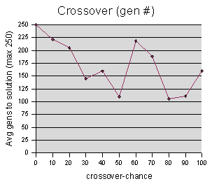
Crossover-chance data were sampled at intervals of 10, averaging 5 runs per sample value.
Again with the “gen #” graph, there is some concern that random noise is drowning out any useful results. However, it is clear from the “best fitness” graph, that very low crossover-chance values adversely affect the genetic programming process. (Note that we are only varying the crossover-chance parameter, while holding clone-chance and mutation-chance constant -- this graph is really studying the triplets (Crossover, Clone, Mutate) = (0,20,10) (10,20,10) (20,20,10) etc.)
 |
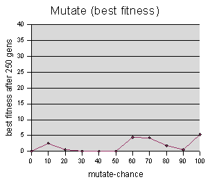 |
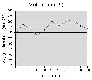
Mutate-chance data were sampled at intervals of 10, averaging 5 runs per sample value.
The data is inconclusive, and I am
hesitant to say anything more about it.
 |
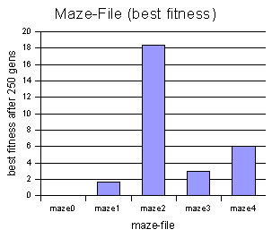 |
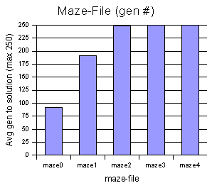
Each
maze file was run 10 times, and
the results were averaged.
|
This test was mostly out of
curiosity,
to see which mazes this model performs better on, and which give it
difficulty.
|
 |