Asynchronous Circuits
Lecture #16 , Feb 14th 2000
Lecture #16 , Feb 14th 2000
Terminology
The fundamental property of a sequential circuit is that the output is a function of input as well as states. The basic problem is that how the past history can be captured. In synchronous circuits clock was responsible for the transfer of state from the Present State to the Next State. But there is no clock in Asynchronous circuits.
Here the notion of a state is a little different. Here the changes in output are initiated by change in inputs ( In sync. Circuits , changes occurred due to the clock ). There are two kinds of variables here : the input variables and secondary variables.
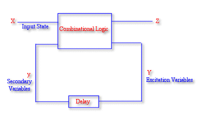
Given a certain state , next state occurs through excitation variations. There is no clock here. The loop shown above is not broken at any point of time , so a series of excitations can circulate. Eventually it will reach a stable secondary state ( Non oscillating ) : Y à Y i.e. Equilibrium State.
If we permit multiple inputs to change simultaneously , then designing the circuit becomes a very complex task so the machine is operated in the Fundamental Mode.
In Fundamental mode , only one input can change at a time. Here the design is much more complex than the sync. Machine.
After designing the machine , we may examine the effect of multiple input changes at a time ( however we can ensure that no subsequent change will occur until all transients die down )
Delay

In the block circuit shown previously , a delay component was shown seperately which is essential for the proper working of the circuit.For asynchronous circuits , fortunately we don. t need any separate component for delay. Combinational logic has its own delay so no special component is required. (We can assume that the combinational logic is ideal and the delay is a separate block )
Illustrative Example
Consider a circuit with 2 input variables x1 and x2 and one output variable z. Output is 1 only when x1=x2=1 , while x1 being 1 first.
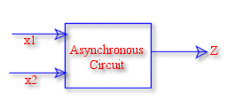
Note : Without the last condition , the circuit essentially becomes a combinational logic problem as no "memory" is required here.
Waveform

It should be so drawn , so that all possible combinations are analysed.
The waveform drawn above is precise because x1 and x2 can. t change simultaneously ( Fundamental Mode )
After drawing the waveform , we move onto the next step i.e. identifying the states.
Total States

Here all the states labelled are stable states as no further changes occur if no input changes occur.
Note that the State 5 and State 3 shown above are different because output z is different for these inputs ( Secondary variables are different while the input variables are the same )
The states may be different even if the inputs and outputs are same , under some cases ( To be discussed in the next class )
The next step is to tabulate a table known as the The Primitive Flow Table.
The Primitive Flow Table
The primitive flow table shows how the state machine works and how the various states are passed before reaching the stable states. The non-stable states are also known as the transient states.
The general rule to draw the Primitive Flow Table is to follow the waveform drawn previously .
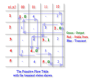
When input changes occurs from 00 to 10 , there is a transient state. Here in the table we say that the transient state is same as the next stable state.
Next step is to consider other 1-input changes possible at each stable state i.e. to consider the effect of adjacent inputs ( of Hamming Distance 1)at each stable state. This makes the Primitive Flow Table complete.
After this the Final Table is drawn.
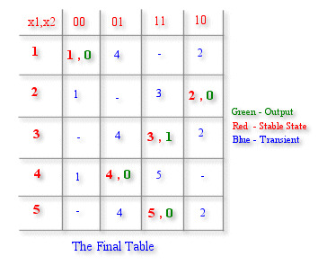
Note : In sync. Machines , we need registers to store the various states ( Here the 5 states are function of both the input and secondary variables )
We now need to know the secondary variables required.
The next step is to build a Merger Graph which essentially portrays the compatibility between the states.
To check compatibility :
Columnwise , if every entry is compatible , then those
rows are compatible ( states should be same , transient & stable
)
The compatible rows in the above table are :
1à 2 1à 3 1à 4 1à 5 2à 3 4à 5
Merger Graph
Cliques are those partitions of the graph which are completely connected.
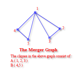
In the above graph , following secondary variables are obtained :
A ( 1,2,3 )
B (4,5)
It should be noted that for the sake of minimisation , no common node should be there in the above partitions. All of this is done to find the minimum no. of secondary states.
Reduced FlowTable
After the Merger Graph step , we get the secondary variables which need to distinguish between the states.
The reduced flow table is got from the previous 5 row state table by combining those rows which form a clique. Then some arrows drawn previously vanish as they travel within one clique. ( i.e. some transients vanish ).
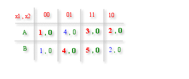
The reduced Flowtable
Here only two secondary states are required à Only 1 variable is needed.
Some transients have vanished due to merging.
Note : When we go from 00 to 01 à transition is there. What about the output ? We choose the output in the transition to be the same as next stable state ( so that the output is present as early as possible )
Now the main task is completed . Only the state assignment is left.
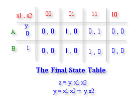
The final state table is got by replacing each state by its corresponding reduced state number which were obtained from the Merger Graph.
The Final State Table
The final circuit
The final circuit is as shown.
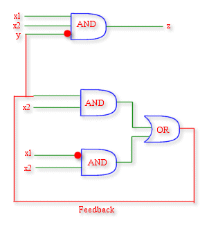
z = y. x1x2
y = x1. x2 + yx2
Further insight can be gained by actually testing it mentally. Following are the outputs z and y when the given inputs are fed to circuit.
|
x1 |
x2 |
z |
y |
|
0 |
0 |
0 |
0 |
|
1 |
0 |
0 |
0 |
|
1 |
1 |
1 |
0 |
|
0 |
1 |
0 |
1 |
|
1 |
1 |
0 |
1 |
In the above table we can see the different conditions produced depending upon different inputs. In complicated situations , various problems may occur such as critical races etc. which will be addressed in the next few lectures.